LSTM Networks for estimating growth rates in DCF Models

The Discounted Cash Flow (DCF) Model: A Brief Overview
In the world of finance, understanding the potential future performance of a company is a crucial endeavor. Investors, analysts, and financial experts rely on various models to estimate a company's valuation to make informed investment decisions. In this article, we will explore the most common valuation models and examine whether LSTM networks can be valuable tools in this context.
The Discounted Cash Flow (DCF) model is broadly used to estimate the intrinsic value of an asset, typically a company or an investment, based on its future cash flows. It helps investors determine whether the current market price of the asset is overvalued or undervalued.
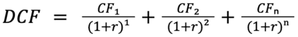
Where:
- CFi represents the expected cash flow in year i;
- r is the discount rate that reflects the time value of money.
The DCF model consists of two main components: Free Cash Flows (FCF) and the Discount Rate. FCF represents the cash generated by a company's core operations that is available for distribution to investors and debt holders after accounting for necessary expenditures. It provides a clearer picture of the cash available for reinvestment, debt reduction, dividends, or other capital allocation decisions. Using FCF in the DCF model provides a more accurate and representative measure of a company's cash flow that is directly linked to its core operations and potential for value creation.
Different approaches can be used to calculate FCF, such as the Free Cash Flow to Equity (FCFE) method or the Free Cash Flow to Firm (FCFF) method. The choice depends on the perspective from which you are evaluating the company and the specific assumptions you are making. The FCFE method is often used when valuing the equity portion of a company, with a focus on the cash flows available to the company's equity shareholders. The FCFF method is applied when valuing the entire firm, irrespective of the mix of debt and equity financing.
The Discount Rate is used to account for the time value of money and risk, and is often calculated using the Weighted Average Cost of Capital (WACC) or the Cost of Equity.
Forecasting Growth of DCF Components
One of the primary challenges in the DCF model is accurately forecasting the growth rates of its FCF components. There are various methods, each with its own strengths and limitations:
- Historical Growth Rates: This method involves analyzing a company's past growth rates and extrapolating them into the future. However, historical trends may not accurately represent future growth dynamics, especially if the company's industry or competitive landscape changes.
- Analyst Projections: Analysts provide growth rate estimates based on their research and analysis. While valuable, these projections can vary widely among analysts and might not capture unexpected shifts in market conditions.
- Industry Growth Rates: Using industry benchmarks can provide insight into a company's growth potential relative to its peers. However, industries can experience sudden disruptions that render historical growth patterns less relevant.
- Regression-Based Approaches: Statistical regression models use historical data to predict future growth. These models assume that historical relationships will persist, but they may not account for changing business dynamics.
These methods often have limitations and may not capture complex patterns or sudden changes in growth. Recognizing these limitations, the proposed solution is to leverage Long Short-Term Memory (LSTM) networks—a form of artificial neural networks—to enhance growth rate forecasts. LSTMs are designed to capture intricate temporal patterns and adapt to changing conditions, making them promising tools for forecasting complex growth dynamics more accurately. By utilizing LSTM networks, analysts aim to bridge the gap between traditional forecasting methods and the nuanced realities of today's business landscape, where growth patterns are influenced by a myriad of factors. The use of advanced technologies like LSTMs offers the potential to capture sudden changes, cyclical patterns, and non-linear trends that may elude conventional forecasting approaches. As a result, this approach can lead to more precise growth rate predictions, which are fundamental to accurate valuations in financial analysis.
Introducing Long Short-Term Memory (LSTM) Networks
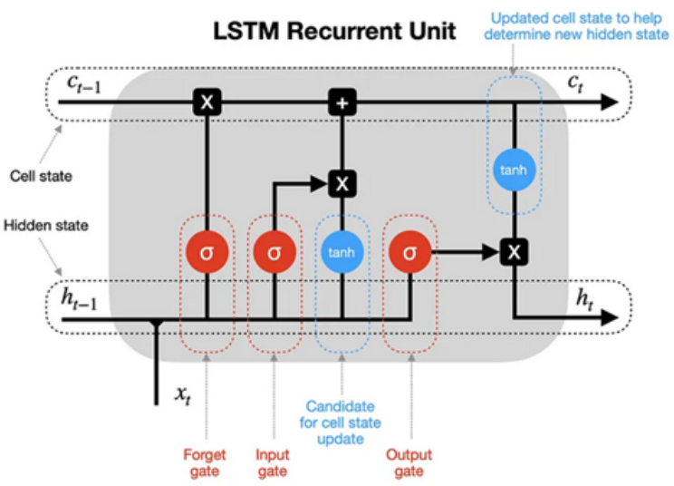
LSTM networks are a type of recurrent neural network (RNN) designed to capture patterns in sequences of data. Unlike traditional feedforward neural networks, LSTMs have a unique memory cell that can store and retrieve information over varying time intervals. This property makes LSTMs particularly effective for time-series data, such as financial data, where patterns and dependencies can span different time frames.
LSTMs consist of three key components:
- Cell State: This is the memory aspect of the LSTM. It carries information through time steps and is modified using gating mechanisms to control the information flow.
- Hidden State: At each time step, it carries information from the previous step to the current one, allowing the network to capture temporal dependencies.
- Gates: LSTMs have three gates - the input gate, forget gate, and output gate. These gates control the flow of information into and out of the cell state, allowing the network to decide which information to keep, forget, or output.
Comparison of Historical Growth Rate Methods and LSTM Model
Let's compare growth rate estimates for next year's Revenue, Capex, Depreciation, and Amortization using Historical Growth Rate methods and LSTM model.
For training the LSTM model, we use the company's time series data from the past 7 years, which includes Revenue, Capital Expenditures, and Depreciation and Amortization. For each time point, we take the latest available value of each metric over the trailing twelve months and normalize it by the asset value at that time, to account for the company's scale. The resulting time series (approximately 1750 points) is then centered around a mean of 0 and scaled to have a standard deviation of 1.
The target values for training are the normalized values of the metrics for the following year, adjusted by the current asset values. These values are then standardized using historical time series data to estimate mean and standard deviation. The training datasets include time series data from the last 5 years for each metric (Revenue, Capital Expenditures, Depreciation, and Amortization) across all companies.
After training the three models, we denormalize the forecasts based on the current asset values. From the denormalized values, we then calculate the growth rates for the upcoming year.
To estimate growth rates using the historical method, we use the companies' data from the past 7 years, taking the trailing twelve-month periods to calculate annual growth rates. Then we determine the median value from that past seven-year period and use it as the estimated growth rate for the next year.
The table below represents the metric evaluations of Mean Squared Error (MSE), Mean Absolute Error (MAE), and Coefficient of Determination (R-squared) for the growth rate forecasts of both methods relative to the actual growth rate for the next year:
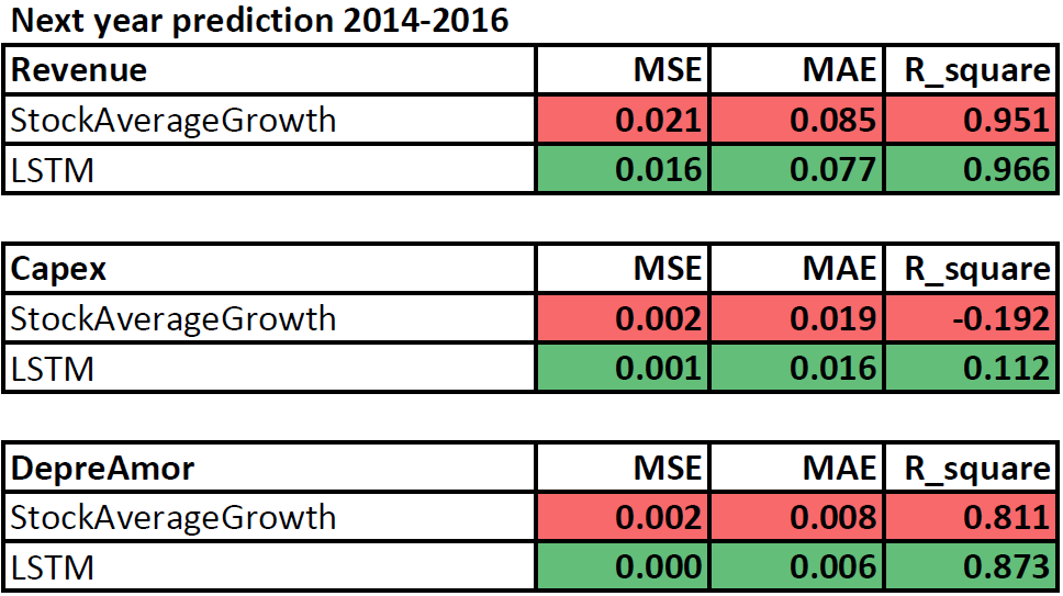
As we can see, the LSTM network's estimates outperformed the historical average growth rate estimates for all metrics.
Sample ranking strategy based on forecasts of growth rates from the LSTM model
We will estimate the company's value using the Discounted Cash Flow (DCF) model, utilizing the derived growth rates to estimate the Free Cash Flow to Firm (FCFF). We will be using NOPAT method where FCFF = NOPAT + D&A - INCREASE in NWC - CapEx.
The primary approach for estimating the growth rate of FCFF components over the next n years begins by assuming that the initial growth rate will transition to the industry average over that period. For the initial rate, we utilize the LSTM estimates from the first year and then linearly interpolate them to the industry growth rates over the subsequent 5 years. By following this approach, we determine the company's valuation using the DCF model.
The proposed strategy is the following: At the beginning of each month, we calculate the upside relative to market capitalization using the formula Upside = DCF value / MarketCap. After sorting all stocks into deciles based on the size of their upside, we purchase stocks from the top three deciles and hold them until the next month's rebalancing. The results relative to SP500 Index are provided in the table below.
| Sharpe | CAGR | Volatility | |
| SnP | 0.55 | 10.8% | 19.7% |
| DCF | 0.75 | 13.8% | 18.5% |
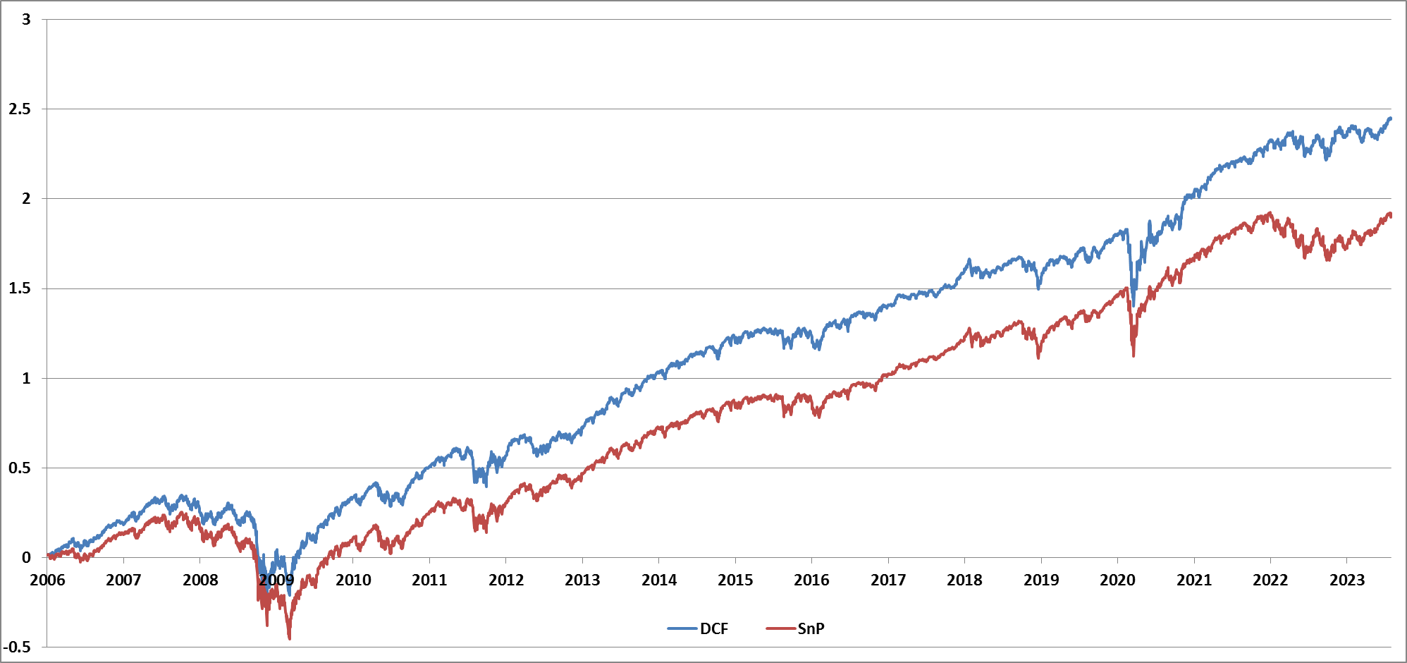
From the data above, we can see that the ranking strategy, which utilizes the Upside metric from DCF valuations, demonstrates superior performance compared to market returns. By achieving more precise growth rate estimates for the Free Cash Flow components, we gain a deeper insight into a company's financial trajectory over subsequent years. This insight can add value and help investors to make more informed decisions. Implementing neural networks, particularly LSTM, offers a viable solution to this challenge and stands as a valuable alternative to conventional methods.